2048

It's been a while without any new posts here; I've been focused on projects where JavaScript or C are more suitable than Haskell (for me, anyway). But I did dust off GHC this weekend to write this no-frills clone of Gabriele Cirulli's popular '2048' puzzle game. It didn't come out quite as concise as I had hoped - maybe I'm a bit rusty? :)

As usual with my graphical stuff, you'll need the legacy (1.2) versions of SDL to compile this. And the font path may vary; adjust it for your system.

	import Control.Monad
	import Data.List (notElem, nub, transpose, unfoldr)
	import Graphics.UI.SDL as SDL
	import Graphics.UI.SDL.TTF as TTF (init, openFont, renderTextSolid)
	import System.Random.Mersenne.Pure64 (newPureMT, randomInt)
	-------------------------------------------------------------------
	[xres, yres] = [512, 512]
	main = withInit [InitVideo] $ do
	TTF.init
	window <- setVideoMode xres yres 32 []
	seeds <- replicateM 2 newPureMT
	board <- initBoard $ randCoords seeds
	dejaVu <- openFont font 48
	enableEvent SDLMouseMotion False
	setCaption "2048" "2048"
	run window dejaVu board $ randCoords seeds
	where
	font = "/usr/share/fonts/TTF/liberation/LiberationMono-Bold.ttf"
	run w font grid (p:ps) = do
	delay 32
	when (0 `notElem` concat grid) endGame
	render w font grid
	e <- pollEvent
	case e of
	KeyUp (Keysym SDLK_ESCAPE _ _) -> endGame
	KeyUp (Keysym SDLK_UP _ _) -> go (f $ up grid) ps
	KeyUp (Keysym SDLK_RIGHT _ _) -> go (f $ right grid) ps
	KeyUp (Keysym SDLK_DOWN _ _) -> go (f $ down grid) ps
	KeyUp (Keysym SDLK_LEFT _ _) -> go (f $ left grid) ps
	_ -> go grid $ p:ps
	where
	endGame = showScore w font . sum $ map sum grid
	(go, f) = (run w font, birth $ p:ps)
	birth (p:ps) m = if zero p then set m p 2 else birth ps m
	where
	zero (i,j) = 0 == (m !! j) !! i
	render w font grid = do
	fillRect w (Just $ Rect 0 0 xres yres) bgBlue
	digits <- zipWithM txtify grid' color
	zipWithM_ (draw w) digits windowCoords
	SDL.flip w
	where
	txtify = renderTextSolid font . text
	text n = if n == 0 then " " else show n
	color = repeat $ Color 255 255 100
	grid' = concat $ transpose grid
	bgBlue = Pixel 0xFF112277
	showScore w font score = do
	fillRect w (Just $ Rect 0 0 xres yres) (Pixel 0)
	let s = "Score: " ++ show score
	txt <- renderTextSolid font s $ Color 255 255 255
	draw w txt (140 - 10 * length (show score), 220)
	SDL.flip w >> SDL.delay 3500 >> SDL.quit
	draw w s p = blitSurface s Nothing w $ rect p
	where
	rect (x,y) = Just $ Rect x y 1 1
	----------------------------------------------
	wrap = take 4 . merge . (++ repeat 0)
	where
	merge (m:n:ns)
	| m == n = 2 * m : merge ns
	| m /= n = m : merge (n:ns)
	left = map wrap . pull
	right = map (reverse . wrap . reverse) . push
	up = transpose . map wrap . transpose . raise
	down = transpose . f . transpose . lower
	where
	f = map $ reverse . wrap . reverse
	(raise, lower) = (xfx pull, xfx push)
	where
	xfx f = transpose . f . transpose
	(push, pull) = (map $ fst . f, map $ snd . f)
	where
	f ns = (blanks ++ r, r ++ blanks)
	where
	blanks = replicate (4 - l) 0
	(r, l) = (filter (> 0) ns, length r)
	----------------------------------------------
	initBoard ps = return $ set (set grid p 2) q 2
	where
	grid = replicate 4 [0,0,0,0]
	[p,q] = take 2 . nub $ take 10 ps
	randCoords [g, g'] = zip xs ys
	where
	xs = f $ unfoldr (Just . randomInt) g
	ys = f $ unfoldr (Just . randomInt) g'
	f = map (`mod` 4)
	windowCoords = liftM2 (,) ns ns
	where
	ns = [32, 160, 288, 416]
	set m (i,j) v = take j m ++ val : xs
	where
	(val, xs) = (f (m !! j) i v, drop (j+1) m)
	f xs i v = take i xs ++ (v : drop (i+1) xs)

view raw 2048.hs hosted with ❤ by GitHub

ramanujan's Π summation

When G.H. Hardy first began his correspondence with Srinivasa Ramanujan, he was amazed by the prodigy's elegant and surprising series for irrational and transcendental values. Although Ramanujan hadn't included proofs of the theorems, Hardy told his colleagues, "they must be true, because, if they were not true, no one would have the imagination to invent them."

For example, here's Ramanujan's sum for Π which, after just 3 terms, overwhelms IEEE 754 double precision. Modern discoveries, like spigot algorithms on non-decimal bases, can find a given individual digit in constant time. But for fully expanding Π, no one has surpassed Ramanujan's expression: both the Chudnovsky brothers and Yasumasa Kanada adapted it to achieve their milestone calculations.

	import Prelude hiding (pi)
	pi = recip . sum $ map f [0..2]
	f k = a * (b / c)
	where
	a = (2 * sqrt 2) / 9801
	b = fac (4 * k) * (1103 + 26390 * k)
	c = fac k**4 * (396**(4 * k))
	fac n = product [1..n]

view raw ramanujan_PI.hs hosted with ❤ by GitHub

generalizing langton's ant

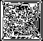
Christopher Langton's ant can be generalized by adding states to the ant, producing automata known as turmites. Shown here is the behavior of one interesting two-state turmite, started on an empty plane. Click the thumbnail to see more generations; you'll see that this turmite always produces a framed square with the same distinctive irregular pattern.

	import Control.Arrow ((***))
	import Control.Monad (join, void, when)
	import Data.Set (delete, empty, insert, member, toList)
	import Graphics.UI.SDL as SDL
	(xres, yres, sq) = (1600, 900, 2)
	main = withInit [InitVideo] $ do
	w <- setVideoMode xres yres 32 [NoFrame]
	enableEvent SDLMouseMotion False
	setCaption "Turmite" "Turmite"
	run w [1..] 0 p (0,1) empty
	where
	p = (xres `div` 2 `div` sq, yres `div` 2 `div` sq)
	run w (n:ns) s p v ps = do
	when (n `mod` 23 == 0) $ render w ps
	e <- pollEvent
	case e of
	KeyUp (Keysym SDLK_ESCAPE _ _) -> print n >> printout
	KeyUp (Keysym SDLK_SPACE _ _) -> pause w s p v ps
	_ -> continue
	where
	continue = go w ns s p v ps
	printout = void $ saveBMP w "output.bmp"
	pause w s p v ps = do
	delay 128
	e <- pollEvent
	case e of
	KeyUp (Keysym SDLK_ESCAPE _ _) -> return ()
	KeyUp (Keysym SDLK_SPACE _ _) -> run w [1..] s p v ps
	_ -> pause w s p v ps
	render w ps = do
	fillRect w (Just $ Rect 0 0 xres yres) $ Pixel 0
	mapM_ (draw w . join (***) (* sq)) $ toList ps
	SDL.flip w
	draw w p = f p =<< g [SWSurface] sq sq 32 0 0 0 0
	where
	rect x y = Just $ Rect x y sq sq
	g = createRGBSurface
	f (x,y) s = do fillRect s (rect 0 0) $ Pixel 0xFFFFFF
	blitSurface s (rect 0 0) w $ rect x y
	go w ns s p v ps
	| s == 0 && not b = run w ns 0 (f p $ l' v) (l' v) qs
	| s == 0 && True = run w ns 1 (f p $ r' v) (r' v) qs
	| s == 1 && not b = run w ns 0 (f p $ r' v) (r' v) rs
	| otherwise = run w ns 1 (f p $ l' v) (l' v) rs
	where
	b = member p ps
	(qs, rs) = (insert p ps, delete p ps)
	f (x, y) = (x +) *** (+ y)
	r' (0, y) = (-y, 0)
	r' (x, y) = ( y, x)
	l' (0, y) = ( y, 0)
	l' (x, y) = ( y, -x)

view raw langton_turmite.hs hosted with ❤ by GitHub

gumowski-mira attractor

Here's an unusual chaotic attractor: the web doesn't seem to have much information on this one, except that it was invented to model particle trajectories in physics. A google image search for 'mira fractals' does turn up some pretty results though.

The system seems to give interesting results only when b is close to one. It behaves less chaotically when b > 1 is fixed, so you can actually animate it - click the thumbnail to see.

	import Control.Arrow ((***))
	import Graphics.UI.SDL as SDL
	(xres, yres) = (200, 200)
	main = withInit [InitVideo] $ do
	w <- setVideoMode xres yres 32 [NoFrame]
	enableEvent SDLMouseMotion False
	setCaption "Gumowski-Mira" "Gumowski-Mira"
	loop w p pss
	where
	p = (xres `div` 2, yres `div` 2)
	pss = map points [0.31, 0.3101.. 0.316]
	loop w p pss = do
	render w p $ map (round *** round) $ head pss
	e <- pollEvent
	case e of
	KeyUp (Keysym SDLK_ESCAPE _ _) -> return ()
	_ -> loop w p $ tail pss
	render w (x,y) ps = do
	s <- createRGBSurface [SWSurface] 2 2 32 0 0 0 0
	fillRect w (Just $ Rect 0 0 xres yres) (Pixel 0)
	mapM_ (draw s 0xFFFFFF . rect . center) ps
	SDL.flip w
	where
	center = ((xres - x) +) *** (+ (yres - y))
	rect (x,y) = Just $ Rect x y 1 1
	draw s c p = do fillRect s Nothing $ Pixel c
	blitSurface s Nothing w p
	points a = take 650000 . map (h *** h) $ iterate f (12, 0)
	where
	f (x,y) = let x' = b*y + g x in (x', -x + g x')
	g x = a*x + (2 * (1 - a) * x^2) / (1 + x^2)
	(b,h) = (1.005, (* 4))

view raw gumowski-mira.hs hosted with ❤ by GitHub

128-bit AES electronic codebook

Rijndael (the core of AES) is an algorithm that might actually be shorter and simpler in C, but I was curious to see how natural I could make it look in Haskell. Thanks to Jeff Moser and Sam Trenholme for their clear elucidations.

Note that this code only does ECB mode; it computes rather than hard-codes the S-box; and it could be vulnerable to side-channel attacks. So enjoy reading it, but don't try to make a serious encryption app out of it. That kind of thing is best left to the professionals :)

	{-# LANGUAGE NoMonomorphismRestriction #-}
	import Control.Applicative (liftA2)
	import Data.Bits (xor, shiftL, shiftR, (.|.), (.&.))
	import Data.List (transpose, sortBy, foldl')
	import Data.Ord (comparing)
	import Data.Word (Word8)
	encrypt input key = last ks `g` sRows (h t)
	where
	t = foldl1 (g . f) $ init (k : tail ks)
	f = transpose . map mix . transpose . sRows . h
	g = zipWith $ zipWith xor
	h = map $ map sub
	k = input `g` head ks
	ks = expand key
	mix [a,b,c,d] = [a', b', c', d']
	where
	a' = w ⊕ d ⊕ c ⊕ x ⊕ b
	b' = x ⊕ a ⊕ d ⊕ y ⊕ c
	c' = y ⊕ b ⊕ a ⊕ z ⊕ d
	d' = z ⊕ c ⊕ b ⊕ w ⊕ a
	[w,x,y,z] = map fg [a,b,c,d]
	fg b = b''
	where
	b' = shiftL b 1
	b'' = ((b .&. 0x80) == 0x80) ? (b' ⊕ 0x1B, b')
	sRows (w:ws) = w : zipWith f ws [1,2,3]
	where
	f w i = take 4 $ drop i $ cycle w
	-----------------------------------------------------------
	expand k = scanl f k [1, 2, 4, 8, 16, 32, 64, 128, 27, 54]
	where
	f n w = xpndE (transpose n) . xpndC . xpndB . xpndA $ xpnd0 w n
	xpndE n [a,b,c,_] = transpose [a, b, c, zipWith xor c $ last n]
	xpndC [a,b,c,d] = [a, b, zipWith xor b c, d]
	xpndB [a,b,c,d] = [a, zipWith xor a b, c, d]
	xpndA [a,b,c,d] = zipWith xor a d : [b,c,d]
	xpnd0 rc ws = take 3 tW ++ [w']
	where
	w' = zipWith xor (map sub w) [rc, 0, 0, 0]
	tW = transpose ws
	w = take 4 $ tail $ cycle $ last tW
	----------------------------------------------------
	sub w = get sbox (fromIntegral lo) $ fromIntegral hi
	where
	(hi, lo) = nibs w
	nibs w = (shiftR (w .&. 0xF0) 4, w .&. 0x0F)
	(⊕) = xor
	p ? (a,b) = if p then a else b; infix 2 ?
	get wss x y = (wss !! y) !! x
	----------------------------------------------------
	sbox = grid 16 $ map snd $ sortBy (comparing fst) $ sbx 1 1 []
	sbx :: Word8 -> Word8 -> [(Word8, Word8)] -> [(Word8, Word8)]
	sbx p q ws
	| length ws == 255 = (0, 0x63) : ws
	| otherwise = sbx p' r $ (p', xf ⊕ 0x63) : ws
	where
	p' = p ⊕ shiftL p 1 ⊕ ((p .&. 0x80 /= 0) ? (0x1B, 0))
	q1 = foldl' (liftA2 (.) xor shiftL) q [1, 2, 4]
	r = q1 ⊕ ((q1 .&. 0x80 /= 0) ? (0x09, 0))
	xf = r ⊕ rotl8 r 1 ⊕ rotl8 r 2 ⊕ rotl8 r 3 ⊕ rotl8 r 4
	grid _ [] = []
	grid n xs = take n xs : grid n (drop n xs)
	rotl8 w n = (w `shiftL` n) .|. (w `shiftR` (8 - n))

view raw rijndael-AES.hs hosted with ❤ by GitHub

butterfly curve

Temple Fay discovered this complicated curve in 1989. It can be defined either parametrically or as a polar equation; I did it the former way.

One application I thought of for this is object motion in games: I tried it out by writing this little Canvas game, where the comets follow the curve's trajectory. The differences in plot density along the curve create natural-looking comet tails.

	{-# LANGUAGE NoMonomorphismRestriction #-}
	import Data.Bits ((.|.), shiftL)
	import Control.Arrow ((***), (&&&))
	import Graphics.UI.SDL as SDL
	import Graphics.UI.SDL.Primitives (pixel)
	(xres, yres, zz) = (1050, 1050, round *** round)
	main = withInit [InitVideo] $ do
	w <- setVideoMode xres yres 32 [NoFrame]
	enableEvent SDLMouseMotion False
	setCaption "Butterfly Curve" "Butterfly Curve"
	fillRect w (Just $ Rect 0 0 xres yres) $ Pixel 0
	plot w $ center $ scale curve
	loop w []
	where
	scale = map ((150 *) *** (* 150))
	center = map (((xres / 2) +) *** (+ ((yres + 190) / 2)))
	curve = map (f &&& (negate . g)) ts
	where
	ts = [-999, -998.99.. 999]
	f t = sin t * (e ** cos t - 2 * cos (4*t) - h (t / 12))
	g t = cos t * (e ** cos t - 2 * cos (4*t) - h (t / 12))
	h = foldr1 (.) $ replicate 5 sin
	e = exp 1
	plot w = mapM_ (f . zz)
	where
	f (x,y) = pixel w (fromIntegral x) (fromIntegral y) $ Pixel rgb
	where
	rgb = rgb' .|. shiftL (255 `div` (max x y `div` min x y)) 8
	rgb' = rgb'' .|. shiftL (255 `div` (xres `div` x)) 16
	rgb'' = 0xFF .|. shiftL (255 `div` (yres `div` y)) 24
	loop w ps = do
	delay 128
	event <- pollEvent
	case event of
	KeyUp (Keysym SDLK_ESCAPE _ _) -> return ()
	_ -> loop w ps

view raw fay_butterfly_curve.hs hosted with ❤ by GitHub

bézier curves

De Casteljau's algorithm is a fast, numerically stable way to rasterize Bézier curves. This code implements an interactive demo: click to append nodes to the curve's defining polygon, and drag any node to alter the curve.

	{-# LANGUAGE NoMonomorphismRestriction #-}
	import Control.Monad (when)
	import Control.Arrow ((***))
	import Data.List (findIndex)
	import Graphics.UI.SDL as SDL hiding (init)
	import Graphics.UI.SDL.Primitives (circle, line)
	dim = 400
	main = withInit [InitVideo] $ do
	w <- setVideoMode dim dim 32 []
	enableEvent SDLMouseMotion False
	setCaption "Bézier Curves" "Bézier Curves"
	loop w []
	plot w ps = do
	fillRect w (Just $ Rect 0 0 dim dim) $ Pixel 0xFF222255
	mapM_ (f 2 0xFFFFFFFF . zz) [head ps, last ps]
	when b $ mapM_ (f 3 0x888888FF . zz) controls
	when b $ mapM_ (f 2 0xBBBBBBFF . zz) controls
	where
	f r c (x,y) = circle w x y r $ Pixel c
	(b, controls) = (length ps > 2, tail $ init ps)
	limn w [_] = SDL.flip w
	limn w ((a,b):(x,y):ps) = do
	line w a b x y $ Pixel 0xFFFFFFFF
	limn w $ (x,y) : ps
	loop w ps = do
	delay 128
	event <- pollEvent
	case event of
	KeyUp (Keysym SDLK_ESCAPE _ _) -> return ()
	MouseButtonDown x y _ -> click x y
	_ -> loop w ps
	where
	click x y = let p = rr (x,y) in
	case findIndex ((10 >) . dist p) ps of
	Just i -> drag w i ps
	Nothing -> do
	let ps' = p : ps
	plot w ps' >> SDL.flip w
	when (length ps' > 2) $ render w ps'
	loop w ps'
	drag w i ps = do
	delay 16
	(x,y,_) <- getMouseState
	event <- pollEvent
	let ps' = swap i ps $ rr (x,y)
	plot w ps'
	when (length ps' > 2) $ render w ps'
	case event of
	MouseButtonUp x y _ -> loop w ps'
	_ -> drag w i ps'
	render w ps = limn w $ map zz curve
	where
	curve = map (casteljau ps) [0, 0.001.. 1]
	casteljau [p] t = p
	casteljau ps t = casteljau ps' t
	where
	ps' = zipWith (g t) ps $ tail ps
	g t (a,b) (c,d) = (f t a c, f t b d)
	f t a b = (1 - t) * a + t * b
	swap 0 ps p = p : tail ps
	swap i ps p = take i ps ++ p : drop (i+1) ps
	dist (a,b) (c,d) = sqrt $ (a-c)^2 + (b-d)^2
	rr = fromIntegral *** fromIntegral
	zz = round *** round

view raw interactive_bezier.hs hosted with ❤ by GitHub

convex hulls

This code demonstrates the Graham scan, an O(n log n) method for finding the convex hull (smallest enclosing polygon) of a planar point set. It's a great example of exploiting order: it works by sorting the set by angle about a known extreme point, allowing the hull points to be found in linear time.

A variation on the algorithm, noted by A.M. Andrew, sorts the set lexicographically and finds the upper and lower hull chains separately. This 'monotone chain' version is often preferred, since it's easier to do robustly.

	{-# LANGUAGE NoMonomorphismRestriction #-}
	import Control.Arrow ((***))
	import Data.List (maximumBy, delete, sort, sortBy, unfoldr)
	import Data.Ord (comparing)
	import Graphics.UI.SDL as SDL
	import Graphics.UI.SDL.Primitives (filledCircle, line)
	import System.Random.Mersenne.Pure64 (newPureMT, randomDouble)
	res = 250
	main = withInit [InitVideo] $ do
	w <- setVideoMode res res 32 []
	ps <- randPoints
	enableEvent SDLMouseMotion False
	setCaption "Graham Scan" "Graham Scan"
	fillRect w (Just $ Rect 0 0 res res) $ Pixel 0
	limn w $ map (round *** round) $ hull ps
	plot w ps
	pause
	plot w ps = do
	mapM_ (f . (round *** round)) ps
	SDL.flip w
	where
	f (x,y) = filledCircle w x y 1 $ Pixel 0xFFFFFFFF
	limn w ps = f $ ps ++ [head ps]
	where
	f [_] = return ()
	f ((a,b):(x,y):ps) = do
	line w a b x y $ Pixel 0xFF0000FF
	f $ (x,y) : ps
	pause = do
	delay 128
	e <- pollEvent
	case e of
	KeyUp (Keysym SDLK_ESCAPE _ _) -> return ()
	_ -> pause
	hull qs = go (drop 2 ps) $ reverse $ take 2 ps
	where
	o = bottomRightP qs
	ps = o : sortBy (ccw o) (delete o qs)
	go [] qs = qs
	go (p:ps) s@(a:b:qs)
	| ccw a b p /= GT = go (p:ps) $ b:qs
	| otherwise = go ps $ p:s
	ccw (ax, ay) (bx, by) (cx, cy)
	| d < 0 = LT
	| d > 0 = GT
	| True = EQ
	where
	d = (bx - ax) * (cy - ay) - (by - ay) * (cx - ax)
	bottomRightP = maximumBy (comparing snd) . sort
	randPoints = fmap f newPureMT
	where
	f = uncurry zip . splitAt 20 . g
	g = map (* res) . unfoldr (Just . randomDouble)

view raw graham-scan.hs hosted with ❤ by GitHub

more Π obscurantism

Here's an illustration of an approach to Π pointed out by Kevin Brown. Define f(n) as the nearest greater or equal multiple of n-1, then of n-2, etc (yielding OEIS sequence 2491). Then, inverting a result found by Duane Broline and Daniel Loeb, Π = n² / f(n).

But as you can see from the comment, the series converges very slowly!

	main = print $ e**2 / f e e 1
	where
	e = 900000 -- yields 3.1416003...
	f n 1 _ = n
	f n k l = f n' (k - 1) $ n' / k
	where
	n' = head $ dropWhile (< n) $ map (* k) [l..]

view raw kevin_brown_PI.hs hosted with ❤ by GitHub

segment intersection search

Here's a simple method I learned from Gareth Rees for finding the intersection (or parallel / collinear status) of two line segments. Rees credits Ronald Goldman, though I'd imagine the technique goes further back.

	import Control.Arrow ((***))
	import Control.Monad (liftM2)
	import Data.Int (Int16)
	import Data.List (unfoldr)
	import Graphics.UI.SDL as SDL
	import Graphics.UI.SDL.Primitives (line, circle)
	import System.Random.Mersenne.Pure64 (pureMT, randomInt)
	(xres, yres) = (1600, 900)
	(red, white) = (0xFF0000FF, 0xFFFFFFFF)
	main = withInit [InitVideo] $ do
	w <- setVideoMode xres yres 32 []
	enableEvent SDLMouseMotion False
	setCaption "Line Intersection" "Line Intersection"
	run w . take 15 $ filter f segments
	where
	f pq = dist pq < 1000
	run w ss = do
	delay 256
	drawSegs w ss
	let ss' = map (vectorize . cst) ss
	drawPoints w $ liftM2 crossing ss' ss'
	SDL.flip w
	e <- pollEvent
	case e of
	KeyUp (Keysym SDLK_ESCAPE _ _) -> return ()
	_ -> run w ss
	drawSegs w = mapM_ f
	where
	f ((a,b), (c,d)) = line w a b c d $ Pixel red
	drawPoints w = mapM_ (f . (round *** round))
	where
	f (x,y) = circle w x y 5 $ Pixel white
	-------------------------------------------------------
	segments = h $ zip (f xres 13) $ f yres 23
	where
	f m = map (fromIntegral . (`mod` m)) . g . pureMT
	g = unfoldr $ fmap randomInt . Just
	h (p:ps) = (p, head ps) : h (tail ps)
	dist (p,q) = sqrt $ (a-c)^2 + (b-d)^2
	where
	[a,b,c,d] = map f [fst p, snd p, fst q, snd q]
	f = fromIntegral
	crossing (p,r) (q,s)
	| f = p .+. (t .^. r) -- exactly one intersection
	| True = (-5,-5) -- parallel, colinear, etc.
	where
	t = (q .-. p) .*. s / (r .*. s)
	u = (q .-. p) .*. r / (r .*. s)
	f = (r .*. s) /= 0 && h t && h u
	h n = 0 <= n && n <= 1
	(a,b) .+. (c,d) = (a+c, b+d)
	(a,b) .-. (c,d) = (a-c, b-d)
	n .^. (x,y) = (n*x, n*y) -- vector scaling
	(a,b) .*. (c,d) = a*d - b*c -- 2D cross product
	vectorize ((a,b), (c,d)) = ((a,b), (c-a, d-b))
	cst (p,q) = (f p, f q)
	where
	f = fromIntegral *** fromIntegral

view raw line_segment_intersections.hs hosted with ❤ by GitHub

today in oblique approaches

If your standard library offers complex numbers and you're not in any hurry, you can't ask for much simpler (or more obscure!) ways to compute Π than this.

	import Data.Complex (magnitude, Complex((:+)))
	pi = length $ takeWhile (< 2) $ map magnitude zs
	where
	zs = iterate (\z -> z^2 + ((-0.75) :+ 0.0000001)) 0

view raw mandelbrot_PI.hs hosted with ❤ by GitHub

ikeda map

Continuing the theme of strange attractors, here's the well-known one embedded in the Ikeda map. The thumbnail at left shows the central 'vortex' of the attractor, and links to a larger viewport.

In these images, I've plotted the real and imaginary components along the x and y axes respectively. But the more popular way to visualize this attractor adds an extra parameter to the system and is expressed in trigonometric functions. Such adaptation of the code below yields these results.

	{-# LANGUAGE NoMonomorphismRestriction #-}
	import Data.Complex
	import Graphics.UI.SDL as SDL
	(xRes, yRes) = (1366, 768)
	[a, b, k, p] = [0.85, 0.9, 0.4, 7.7]
	main = withInit [InitVideo] $ do
	w <- setVideoMode xRes yRes 32 [NoFrame]
	s <- createRGBSurface [] 1 1 32 0 0 0 0
	fillRect s Nothing $ Pixel 0xFFFFFF
	enableEvent SDLMouseMotion False
	setCaption "Ikeda" "Ikeda"
	render w s $ ikeda $ 0 :+ 0
	SDL.flip w
	run w
	run w = do
	e <- pollEvent
	delay 64
	case e of
	KeyUp (Keysym SDLK_ESCAPE _ _) -> return ()
	_ -> run w
	render w s = mapM_ draw
	where
	rect (x,y) = Just $ Rect (round x) (round y) 1 1
	g (x,y) = (x + xRes / 24, y + yRes / 2.25)
	draw z = blitSurface s Nothing w $ rect $ g p
	where
	p = (1050 * realPart z, 1050 * imagPart z)
	ikeda = take 1500000 . filter g . iterate f
	where
	f z = a + b * z * exp(i * (k-p) * (1 + abs z^2))
	i = 0 :+ 1
	g (r:+i) = -35 < r && r < 35 && -18 < i && i < 18

view raw ikeda-map.hs hosted with ❤ by GitHub

hénon attractor

French astronomer Michel Hénon reported on this strange, fractal attractor in 1976. Since then, it has been among the most studied examples of chaotic dynamical systems.

	{-# LANGUAGE NoMonomorphismRestriction #-}
	import Graphics.UI.SDL as SDL
	(xRes, yRes) = (1366, 768)
	(a, b) = (1.4, 0.3)
	main = withInit [InitVideo] $ do
	w <- setVideoMode xRes yRes 32 [NoFrame]
	s <- createRGBSurface [] 1 1 32 0 0 0 0
	fillRect s Nothing $ Pixel 0xFFFFFF
	enableEvent SDLMouseMotion False
	setCaption "Hénon" "Hénon"
	render w s henon
	SDL.flip w
	run w
	run w = do
	e <- pollEvent
	delay 64
	case e of
	KeyUp (Keysym SDLK_ESCAPE _ _) -> return ()
	_ -> run w
	render w s = mapM_ draw
	where
	rect (x,y) = Just $ Rect (round x) (round y) 1 1
	g (x,y) = (500*x + xRes / 2, 900*y + yRes / 2)
	draw (x,y) = blitSurface s Nothing w $ rect $ g (x,y)
	henon = take 99999 $ filter g $ iterate f (0,0)
	where
	f (x,y) = (1 - a*x^2 + y, b*x)
	g (x,y) = -1.5 < x && x < 1.5 && -0.45 < y && y < 0.45

view raw michel_henon.hs hosted with ❤ by GitHub

langton's ant

For a round of code golf, I wrote this spare implementation of Chris Langton's remarkably simple universal computer. If you want amenities like pause, random starting pattern or even quit, check out this more complete version.

	import Control.Arrow ((***))
	import Control.Monad (when, join)
	import Data.Set (insert, delete, member, empty)
	import Graphics.UI.SDL as SDL
	(xres, yres, sq) = (1366, 768, 4)
	main = withInit [InitVideo] $ do
	w <- setVideoMode xres yres 32 [NoFrame]
	enableEvent SDLMouseMotion False
	setCaption "Langton's Ant" "Langton's Ant"
	run w [1..] p (0,1) empty
	where
	p = (xres `div` 2 `div` sq, yres `div` 2 `div` sq)
	run w (n:ns) p v ps = do
	when (n `mod` 7 == 0) render
	run w ns (move p $ g v) (g v) $ f p ps
	where
	b = member p ps
	(f,g) = if b then (delete, fl) else (insert, fr)
	fr (x,y) = if x == 0 then (-y,x) else (y,x)
	fl (x,y) = if x == 0 then (y,x) else (y,-x)
	move (x,y) = (x+) *** (+y)
	render = do
	fillRect w (Just $ Rect 0 0 xres yres) $ Pixel 0
	mapM_ (draw w . join (***) (* sq)) ps
	SDL.flip w
	draw w p = f p =<< g [SWSurface] sq sq 32 0 0 0 0
	where
	rect x y = Just $ Rect x y sq sq
	g = createRGBSurface
	f (x,y) s = do fillRect s (rect 0 0) $ Pixel 0xFFFFFF
	blitSurface s (rect 0 0) w $ rect x y

view raw langton_ant.hs hosted with ❤ by GitHub

connett circles

Like Barry Martin's 'Hopalong' fractal, this dynamical system from John Connett was first published in Scientific American in 1986. This demo is interactive: successively clicking two points specifies a rectangle to zoom into. Doing so, you'll see that the system isn't actually a fractal. Instead of self-similarity, deep zooms reveal peacock-like images.

	{-# LANGUAGE NoMonomorphismRestriction #-}
	import Data.Complex (magnitude, Complex((:+)))
	import Graphics.UI.SDL as SDL
	(xres, yres, cast) = (768, 768, fromIntegral)
	main = withInit [InitVideo] $ do
	w <- setVideoMode xres yres 32 [NoFrame]
	enableEvent SDLMouseMotion False
	setCaption "Connett Circles" "Connett Circles"
	zoom w (-2000, -2000) (2000, 2000)
	zoom w (x,y) (s,t) = do
	let r = area x s y t
	render w r
	run w r (0,0)
	run w (xs,ys) p@(x,y) = do
	delay 32
	e <- pollEvent
	case e of
	KeyUp (Keysym SDLK_ESCAPE _ _) -> return ()
	MouseButtonUp i j _ -> click $ f i j
	_ -> run w (xs,ys) p
	where
	f i j = (xs !! cast i, ys !! cast j)
	click q
	| p == (0,0) = run w (xs,ys) q
	| otherwise = zoom w p q
	render w r = draw w . concat . f $ set r
	where
	f = zipWith zip $ map (zip [0..] . repeat) [0..]
	draw w r = do
	s <- createRGBSurface [] 1 1 32 0 0 0 0
	mapM_ (draw s) r
	SDL.flip w
	where
	rect (x,y) = Just $ Rect x y 1 1
	draw s (p,n) = do fillRect s Nothing $ Pixel $ rgb n
	blitSurface s Nothing w $ rect p
	------------------------------------------------------
	rgb n
	| m `mod` 7 == 0 = 0xFFFFFF
	| m `mod` 6 == 0 = 0x00FFFF
	| m `mod` 5 == 0 = 0xFFFF00
	| m `mod` 4 == 0 = 0xFF0000
	| m `mod` 3 == 0 = 0xFF00
	| m `mod` 2 == 0 = 0xFF
	| otherwise = 0
	where
	f x y = round $ magnitude $ (cast x^2) :+ (cast y^2)
	m = abs n
	set (xs, ys) = [[f x y | x <- xs] | y <- ys]
	where
	f x y = round $ magnitude $ (x^2) :+ (y^2)
	area x x' y y' = ([t, t+a.. s], [u, u-b.. v])
	where
	(a,b) = ((s - t) / dx, (u - v) / dy)
	(s,t) = (max x x', min x x')
	(u,v) = (max y y', min y y')
	(dx, dy) = (cast xres, cast yres)

view raw connett_circles.hs hosted with ❤ by GitHub